Fitting exponential decay to beam current data

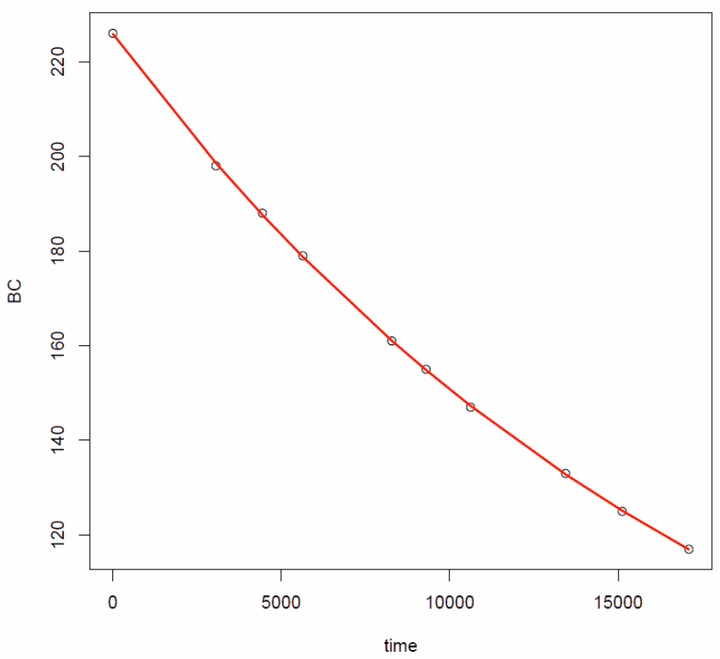
First csv data are imported into R. Then proper formatting of time column is used with strptime function. Then the difference between consecutive time points is calculated (diff function) aa well as cumulative difference in seconds. Finally non-linear fit is performed (with a,k, and b) parameter using function nls. Model coefficient can be extracted by coef function. Finally life time can be obtained from k value tau= (log(2)/k)/3600, and observation points with model curve can be plotted. We can use function with(data, expr, ...) that is a generic R function that evaluates expr in a local environment constructed from data

library(zoo)

#load data

BC <- read.delim("D:/002_R_PROJECTS/2013_09_01_Beam_Current/BC.txt")

#deal with time column
#time difference between the points
z1 <- strptime(BC$Hour, "%H:%M")
dif1=diff(z1)
#cumulative difference in seconds 0 added at the beginning
dif2=data.frame(c(0,60*cumsum(as.numeric(dif1))))
colnames(dif2)=c("time")
BC1 <- data.frame(as.numeric(dif2$time), BC$BC)
colnames(BC1)=c("time","BC")
#non-linear fit
model1 <- nls(BC ~ a*exp(-k*time)+b,data=BC1, start=c(a=240, k=0.0001, b=12)) 
summary(model1)
model.cf <- coef(model1)
a <- model.cf[1]
k <- model.cf[2] 
b <- model.cf[3]  

tau= (log(2)/k)/3600
print(tau)

with(BC1, plot(BC~time))
with(BC1, lines(time, a*exp(-k*time)+b, col="red", lwd =2))